概要
scikit-learnでk近傍法の実演。
@CretedDate 2015/07/12
@Versions Python2.7.6 NumPy1.9.2 scikit-learn0.16.1
テストデータの用意
ランダムな1000件の2次元の座標を用意する。
たかが1000件、されど1000件。すべての要素に対してすべてn件の付近の座標を発見しようとすると、1000×1000で約100万回(実際にはn * (n-1))の距離計算が発生する。
100万なら時間はかかるけど結果は返ってくると思われるので、ブルートフォースで一度頑張って計算してみた後、td木とか使ってより短い時間で計算出来る様子を見てみたい。
普段、pandasを利用しているので、DataFrameに入れてそこから利用するようなコードにする。
import numpy as np
import pandas as pd

df = pd.DataFrame( np.random.random( [1000, 2]) * 100, columns=['x', 'y'] )
df.plot( kind='scatter', x='x', y='y' )
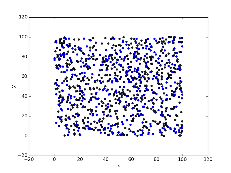
0〜100までに分散した座標が1000個できた。あとはそれぞれの座標に対して、n=10で近い点を探してみる。
ブルートフォース的な処理
まずはブルートフォース的な処理でやってみる。distance metricにはeuclideanを使用。metricにはmanhattan, minkowski, mahalanobis等々が指定できる。詳細はDistanceMetric。
from sklearn.neighbors import NearestNeighbors
import numpy as np

# brouteを指定して計算
nbrs = NearestNeighbors( n_neighbors=10, algorithm='brute', metric='euclidean' ).fit( df[['x', 'y']].values )
distances, indices = nbrs.kneighbors( df[['x', 'y']] )
あれ、一瞬で処理が終わってしまった。1000×1000程度ではダメか。
とりあえずdistancesとindicesが取れる。indicesが各座標のインデックス。distancesがそれぞれに対する距離。
内容を見てみる。
# [0][0]の値を見る
df[['x', 'y']].values[0][0]
  #=> 2.1888346908544687

# [0][0]のindicesの値
indices[0]
  #=> array([  0, 692, 826, 177, 966, 320, 112, 250, 351, 202])

# [0][0]のdistancesの値
distances[0]
  #=> array([ 0.        ,  1.0563636 ,  1.50667912,  1.96711179,  2.43926018,
  #=>         2.45170726,  2.47632366,  4.53019497,  6.67181488,  6.73559722])

# 当該の位置を見てみる
df.ix[0]
  # x     2.188835
  # y    70.459784
df.ix[692]
  # x     1.488012
  # y    71.250197
df.ix[826]
  # x     1.632225
  # y    69.059689
ちゃんと近い座標の点が取れているようだ。
distance的にも、index:0(2.188835, 70.459784)と、index:692(1.488012, 71.250197)のユークリッド距離は
sqrt( (2.188835 - 1.488012) ** 2 + (71.250197 - 70.459784) ** 2 )
で1.0563643253622312なので同値になってる。
結果をplotしてみる。適当に0, 100, 200, 300のnearestな点に対して色を付ける。
ax = df.plot( kind='scatter', x='x', y='y' )
df.ix[ indices[0] ].plot( kind='scatter', x='x', y='y', ax=ax, color='red' )
df.ix[ indices[100] ].plot( kind='scatter', x='x', y='y', ax=ax, color='yellow' )
df.ix[ indices[200] ].plot( kind='scatter', x='x', y='y', ax=ax, color='green' )
df.ix[ indices[300] ].plot( kind='scatter', x='x', y='y', ax=ax, color='orange' )
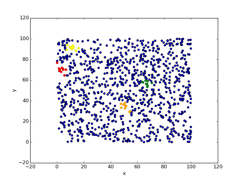
ちゃんと付近が選択されていることがわかる。
td木で速度向上
ブルートフォースすると当然ながら時間がかかるので、事前にtd木を生成して素早く測定できるようにする。といっても、scikit-learnを使う上ではalogrithmにkd_treeと指定するだけなのだけど。
とりあえずbroute指定時の速度計測。
%time nbrs = NearestNeighbors( n_neighbors=10, algorithm='brute', metric='euclidean' ).fit( df[['x', 'y']].values )
  #=> CPU times: user 649 µs, sys: 581 µs, total: 1.23 ms

%time distances, indices = nbrs.kneighbors( df[['x', 'y']] )
  #=> CPU times: user 26 ms, sys: 0 ns, total: 26 ms
体感では一瞬だけど、なにげに26msecもかかっている。
これをkd木にしてみると。
%time nbrs = NearestNeighbors( n_neighbors=10, algorithm='kd_tree', metric='euclidean' ).fit( df[['x', 'y']].values )
  #=> CPU times: user 0 ns, sys: 3.62 ms, total: 3.62 ms

%time distances, indices = nbrs.kneighbors( df[['x', 'y']] )
  #=> CPU times: user 4.06 ms, sys: 0 ns, total: 4.06 ms
当然ながら最初に木を生成するのに2.5msecほど余分に時間がかかっているけど、各distanceの計算は-22msecと大幅に減っている。
ball treeでも同じことをしてみる。
%time nbrs = NearestNeighbors( n_neighbors=10, algorithm='ball_tree', metric='euclidean' ).fit( df[['x', 'y']].values )
  #=> CPU times: user 887 µs, sys: 746 µs, total: 1.63 ms

%time distances, indices = nbrs.kneighbors( df[['x', 'y']] )
  #=> CPU times: user 8.4 ms, sys: 0 ns, total: 8.4 ms
pandasにnearestなn個のindexを登録する
家に着くまでが遠足。DataFrameに格納するまでがPandas使いの処理。
ということで、n個(ここでは5個とする)のindexを入れる処理も書いておく。
indices_df = pd.DataFrame( indices, columns=['n0', 'n1', 'n2', 'n3', 'n4', 'n5', 'n6', 'n7', 'n8', 'n9'] )
df_new = pd.concat( [df, indices_df], axis=1 )

df_new.head()
  #=>            x          y  n0   n1   n2   n3   n4   n5   n6   n7   n8   n9
  #=> 0   2.188835  70.459784   0  692  826  177  966  320  112  250  351  202
  #=> 1  18.636136  20.010189   1  259  366  382  427   71  496  751  766  418
  #=> 2  95.373420  29.524263   2  161  390  844  159  296  399  617  220  153
  #=> 3  71.453374  95.166563   3  525  624  864  834  931  873  914  542  889
  #=> 4  99.907449  10.477509   4  278  711  680  752  372  113  294  662  367
ちょっと適当だけど、まあこれでいいか。