概要
UDFの入ったjarを置くだけでhiveから機械学習的なことができるたいへんお手軽なライブラリ、hivemall。
perceptronやlogistic regressionなどのベーシックなものや、AROWやSCWのような比較的新しいものなどが入っている。Hiveのクエリのみで分類問題が完結できるので、機械学習が専門でない人でもそれなりに扱えそうに見える。
現状では分類と回帰ができて、クラスタリングはできない模様。今回は回帰をちょこちょこやらせてみる。
@Date 2014/08/18
@Versions hivemall v0.2
テストデータを作る
テストデータ生成用の機能も用意されているけど、今回はPythonで生成してtsvファイルにして送ることにする。下記のようなコードで分類しやすそうな点の集まりを生成。
import numpy as np
import pylab as pl

n0 = np.random.normal(loc=1.0, scale=0.7, size=(1000, 2))
n1 = np.random.normal(loc=-1.0, scale=0.7, size=(1000, 2))

pl.scatter( n0[:, 0], n0[:, 1] )
pl.scatter( n1[:, 0], n1[:, 1], color='green' )
pl.show()

label0 = np.zeros( (1000, 1) )
label1 = np.ones( (1000, 1) )

n0 = np.append( label0, n0, 1 )
n1 = np.append( label1, n1, 1 )

np.savetxt("testdata.tsv", np.vstack( (n0, n1) ), delimiter="\t")
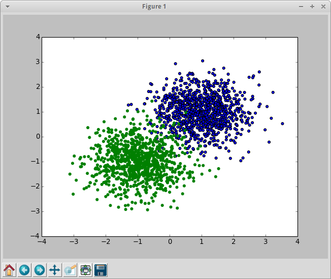
それなりに分類しやすそうで、ある程度は確実に誤りが出る分布。
データはタブ区切りで下記のように出力される。
0.000000000000000000e+00        8.106321700032633748e-01        1.761068673487207192e+00
0.000000000000000000e+00        2.273490165613419656e+00        1.289843946107289696e+00
0.000000000000000000e+00        1.897268010466657495e+00        -6.171459843078190843e-01
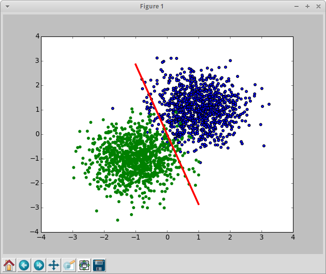
hivemallにお願いする前に、pythonで同じことをやって結果を見ておく。
import numpy as np
import pylab as pl
from sklearn.linear_model import LogisticRegression

n0 = np.random.normal(loc=1.0, scale=0.7, size=(1000, 2))
n1 = np.random.normal(loc=-1.0, scale=0.7, size=(1000, 2))

features = np.vstack( (n0, n1) )
cls = np.concatenate( (np.zeros(1000), np.ones(1000)) )
p = LogisticRegression(fit_intercept=True, penalty='l1', C=0.01)
p.fit( features, cls )

x = [ [-1., -1.], [1., 1.]]
pl.plot( x, p.decision_function( x ), color='red', linewidth=3 )
pl.scatter( n0[:, 0], n0[:, 1] )
pl.scatter( n1[:, 0], n1[:, 1], color='green' )
pl.show()
hivemallに同じことをさせてみる。
hivemallでlogistic regression
hiveに適当なテーブルを作って、生成したファイルを入れる。
CREATE  TABLE `work.hivemall_example`(
  `label` float,
  `x` float,
  `y` float
)
ROW FORMAT DELIMITED
FIELDS TERMINATED BY '\t'
STORED AS TEXTFILE;
load data local inpath 'testdata.txt' into table work.hivemall_example;
データが入ったので、これを分類してみる。jarは既にaddしてあるものとする。概ね下記URLと同じことをしている。
https://github.com/myui/hivemall/wiki/a9a-binary-classification-%28logistic-regression%29
CREATE TABLE work.hivemall_predict
AS
SELECT
  CAST ( feature AS int ) AS feature,
  CAST ( AVG( weight ) AS float ) AS weight
FROM
  (
    SELECT
      logress( addBias(features), label) AS (feature, weight)
    FROM
      (
        SELECT
          label,
          Array(  concat('1:', x), concat('2:', y) ) AS features
        FROM
          work.hivemall_example
      ) t
  ) t
GROUP BY
  feature
するとこんな結果になった。
-1	1.2015901
1	-2.6732762
2	-2.6232412
-1ってなんだろ。あー、biasか。試しにaddbiasせずに実行した場合は、1と2のみになった。
見ての通り最終的には AVG( weight ) とかしているので、複数のMapperで偏りがあった場合なんかに大丈夫なのかは気になるところ。そのためにrand_amplifyとかIterative trainingなどが用意されているらしい。
当然ダメなパターンとかも考えられるけど、気をつければなんとかできそうではある。
さて、predict。今回作ったテーブル構成がJOINしづらいので(反省点)、直で値を書いて誤魔化す。
SELECT
  label,
  x,
  y,
  ( -2.6732762 * x + -2.6232412 * y ) AS total_weight,
  sigmoid( -2.6732762 * x + -2.6232412 * y ) AS prob,
  CAST((case when ( -2.6732762 * x + -2.6232412 * y ) > 0.0 then 1.0 else 0.0 end) as FLOAT) as predict_label
FROM
  work.hivemall_example t
labelとpredict_labelを比較してみる。
SELECT
  COUNT( 1 ),
  SUM( IF ( label = CAST((case when ( -2.6732762 * x + -2.6232412 * y ) > 0.0 then 1.0 else 0.0 end) as FLOAT), 1, 0 ) )
FROM
  work.hivemall_example;
データ的に当然ながら誤りは出る。概ね分類はできている模様。
2000 1955